One possible strategy for trading the financial markets is utilising reinforcement learning algorithms, and frame the
trading task as a "game", where the agent collects rewards for good trades and negative rewards for bad trades.
This particular personal project does a deep dive into common reinforcement learning strategies, before
applying them to the stock market.
Before diving straight into a trading environment, we will sanity check our implementation and tune the function approximator (neural network)
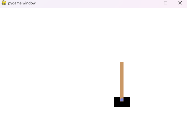
using the well known cartpole game provided by OpenAI Gym/Gymnasium (fig. 1). The code used in this project can be found
here.
Included in the repository is a full set of python unittests which check basic functionality of each of the implemented models to ensure
that the model is working as intended.
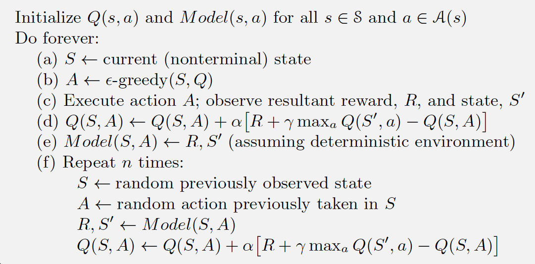
We will be utilizing the Q-learning algorithm (fig. 2), which is an off-policy algorithm (which means it chooses actions in
a different manner compared to the policy the agent is trying to learn) which uses a temporal difference TD(0) update.
When using a neural network to approximate the action-value function (usually denoted with Q(s,a)), the network is
commonly referred to as DQN. The DQN can be augmented in certain ways to produce other variants which can excel under
certain circumstances; namely Double DQN, DynaQ, DynaQ+ and even dueling DQNs (which will not be covered in this project).
We will be testing the efficacy of these models on the aforementioned environment, before eventually moving to predicting optimal trades.
The DQN itself is a very powerful model which was demonstrated to play many Atari games with good results and even achieving super human play
in some games. The Q-learning algorithm can be applied to both tabular and continuous environments, by estimating a value for each possible
action and state combo. The Q-learning update is mathematically proven to converge to the optimal policy under certain conditions; namely that
each state is visited an infinite number of times. However, as we can only train for finite time periods, sometimes the Q-learning agent
can get stuck in a local minima, and one commonly known issue is overestimation. In fact, when performing a deep dive on the DQN using a
basic toy environment which always remains in the same state, with two possible actions, 0 and 1 - where 1 always yields a reward of 1, whereas
the action zero permanently grants zero reward, I observed that the estimated value for action zero often gets overestimated during training, despite
the model never encountering a reward for that action; this is because of the greedy term which takes the maximum value of the value function for the
next state.
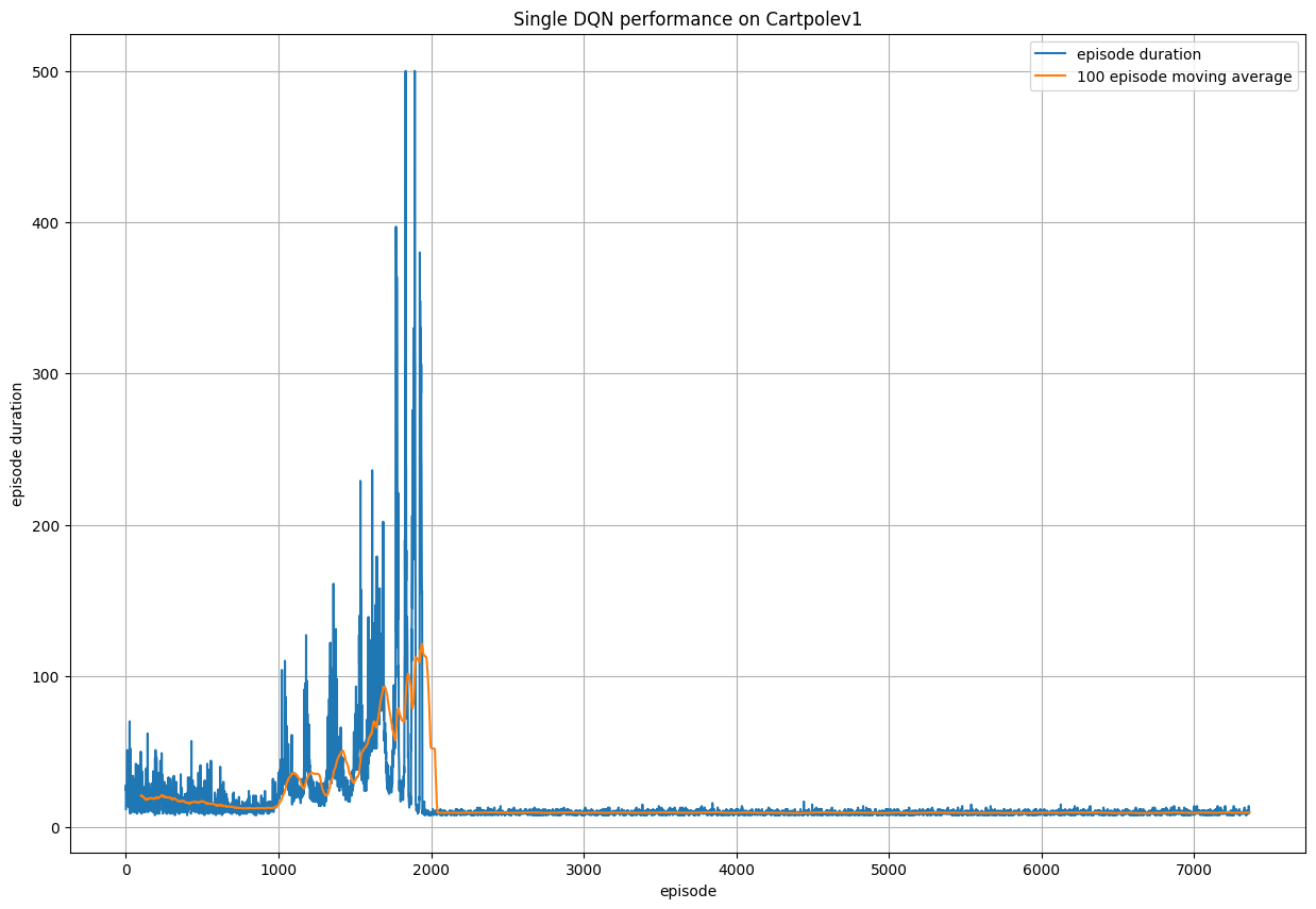
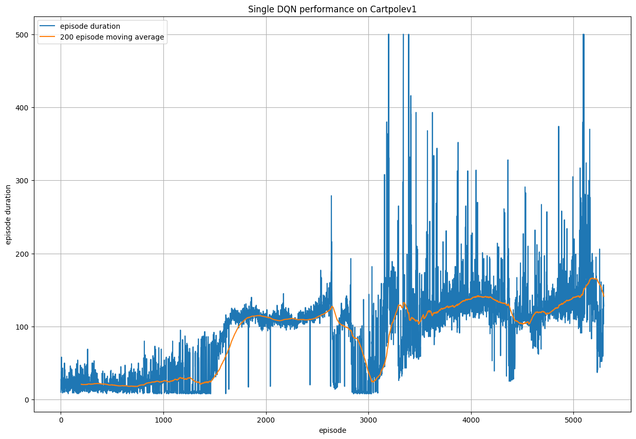
Here we show the reward versus time plots for the DQN itself, and it can be seen that the model is highly unstable and struggles to reach
the optimal policy, even after 5000 episodes of training.
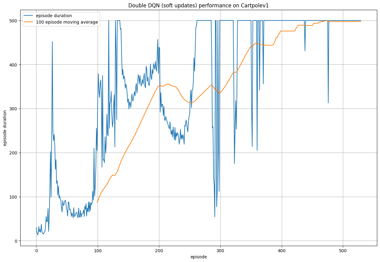
We can augment the DQN model such that we duplicate the Q-network to form a policy network and a target network. The intuition behind this construction is to mitigate the overestimation problem and the "moving target" problem. By fixing the one network and updating the other, we can fix the policy while updating which makes the training much more stable. Obviously the fixed network prediction will be bad initially, but it is updated periodically to match the network that is being updated. Additionally, we experiment with hard and soft updates, which are complete updates at intervals, or small interpolations at each time step.
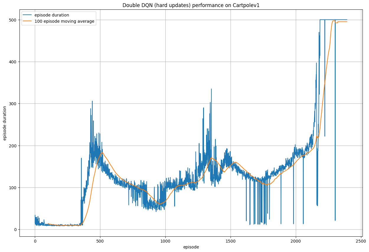
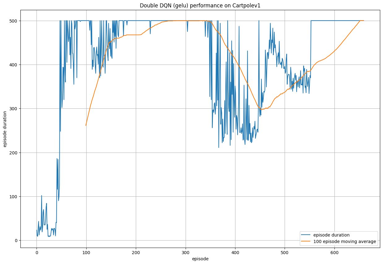
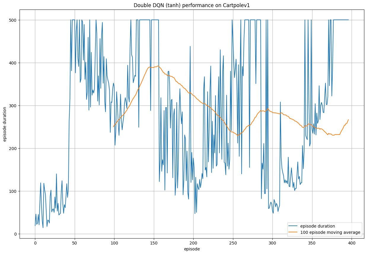
The performance of such agents also changes with different activation functions used within the neural network, and we experiment with ReLU (used in all experiments above), GeLU and Tanh. GeLU exhibits the strongest performance, being a stronger alternative to ReLU in most cases, due to preventing neurons from "dying out".
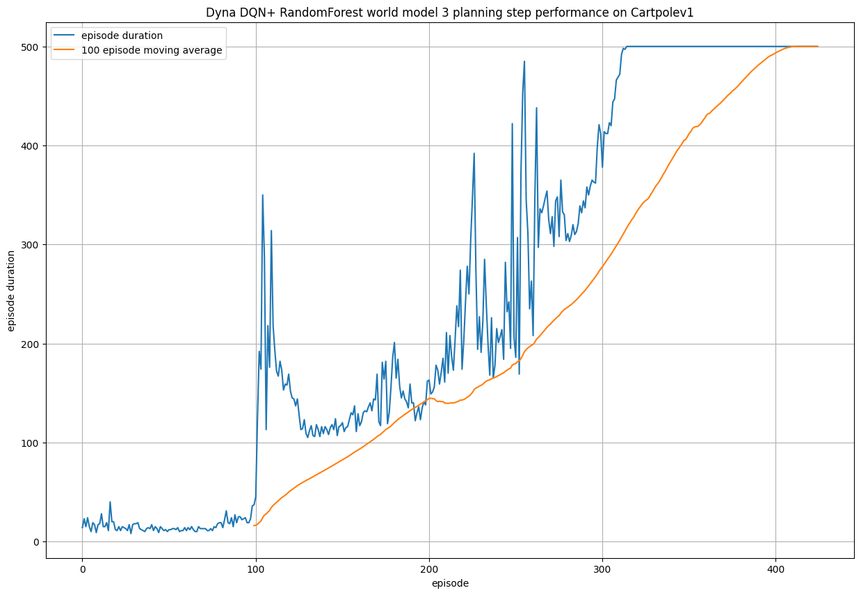
Finally, we test the performance of the DynaDQN algorithm. This is another augmentation of the DQN algorithm, where this time we
simultaneously build a model of the environment internally, which we can use to plan ahead. What this means is past observations are used
to train an internal world model which tries to learn - in this case - a mapping from (state, action) to next state, reward. By doing this, we
can condense our past knowledge into a model which can be used to generate additional fabricated observations which can be used to supplement
actual observations. Every training step that uses these generated observations are called planning steps, and in general, this allows the DynaDQN
to learn the optimal policy from fewer interactions with the environment. This can be useful when interactions with the world is costly. For the world
model we use a random forest regressor.
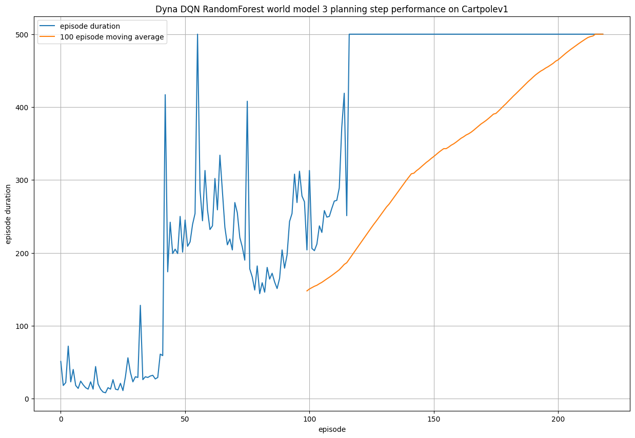
Using 3 planning steps for each actual observation, we can observe that the DynaDQN algorithm training appears more stable and converges to the
optimal policy in less episodes compared to all previous models. Note that the "quality" of such fabricated observations are lower than actual observations
(due to innaccuracies in the world model). So it is important to ensure that not too many planning steps are used.
The last model I implemented is the Dyna Q+ algorithm, which records the last time an action was chosen in a particular state, and uses this to
encourage exploration over time of under trialled actions. This is especially powerful for changing environments as the algorithm is
more inclined to explore new actions if they haven't been used in a while. For this particular task, which uses a static environment, the extra exploration
provides no additional benefit. In fact, the extra exploration of potentially bad actions means that the algorithm takes more episodes to converge to the
optimal policy.
For Trading stocks, the DQN algorithm was trialled using the gym trading environment. We omit the discussion of any Dyna models in this section
as it is well known that modelling stock data is a difficult problem, let alone predicting how each of the individual features transition (modelling
state to state transitions).
These trading gym environments use the exact same methods as the regular
gym environments, but use a user defined dataframe which contains price information of a particular stock. For this task, the data is preprocessed to
include information on some of the most common financial indicators, such as simple moving averages, exponential moving averages, RSI and the MACD. These
are presented alongside price information to the agent, which returns either 1 for buy, 0 for neutral position and -1 for sell. Using the premade
gym environment makes it easy to train on multiple stocks. In this example we try training a DQN algorithm on AAPL, AMZN and GOOG stock prices for the last
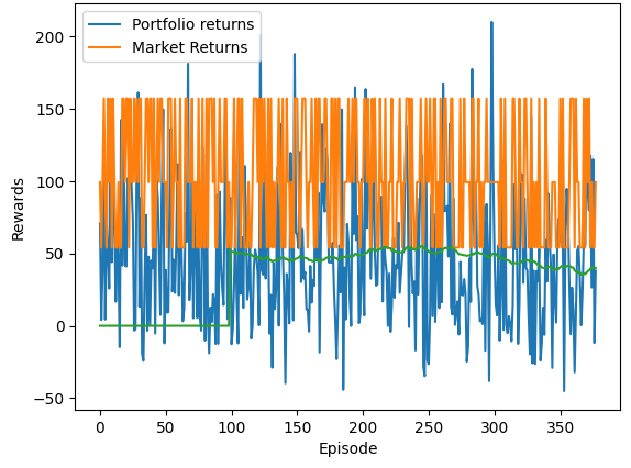
1000 days or roughly three years. The results show that it is not trivial to use a RL agent to trade on regular price data. The quality of the data, the changing
distribution of data, as well as the low signal to noise ratio makes it very difficult to ascertain any concrete patterns in the data. We can see that over time
as the model trains, the performance (portfolio returns over market) still remains very low.
For this research project, I was partnered with the Huawei Neuromorphic Computing Group in Zurich. I was granted use of the Huawei Computing cluster. Workloads were managed using Simple Linux Utility for Resource Management (SLURM). Additionally, in order to train models overnight/long durations, it was essential to use tmux (terminal multiplexer) which kept programs running regardless of whether the local machine is connected or not. In order to utilize the maximum potential of the nodes, it was important to become acquainted with these esoteric systems. Almost all models run in the experiments in this project were created by myself using Pytorch. Public implementations were only used where necessary to verify my own implementation and results. This was a conscious choice to embrace every learning opportunity possible.
Abstract:
It has long been known that Short-Term memory is a key component of the human brain, used for learning skills for one-time or periodic use. This skill is also useful
in language modelling, as oftentimes themes or topics of a corpus of text appear and reappear throughout an article, necessitating the need for the element of forgetting
in language models, which is not currently present. By utilizing ideas presented in recent works about the Short-Term Plasticity Neuron (STPN) and the Linearized Transformer,
we present a new language model, named the STPN-transformer (STPNt), which builds on the idea of the Linearized Transformer by augmenting it with learning to learn and forget.
Experimental results demonstrate the advantages of the STPNt over the Linear Transformer in limited memory settings on the Wikitext-2 dataset. Our research in this thesis begins
to demonstrate some of the potential advantages that this type of learning can provide in language modelling, to be built on in future works.
Contributions to field:
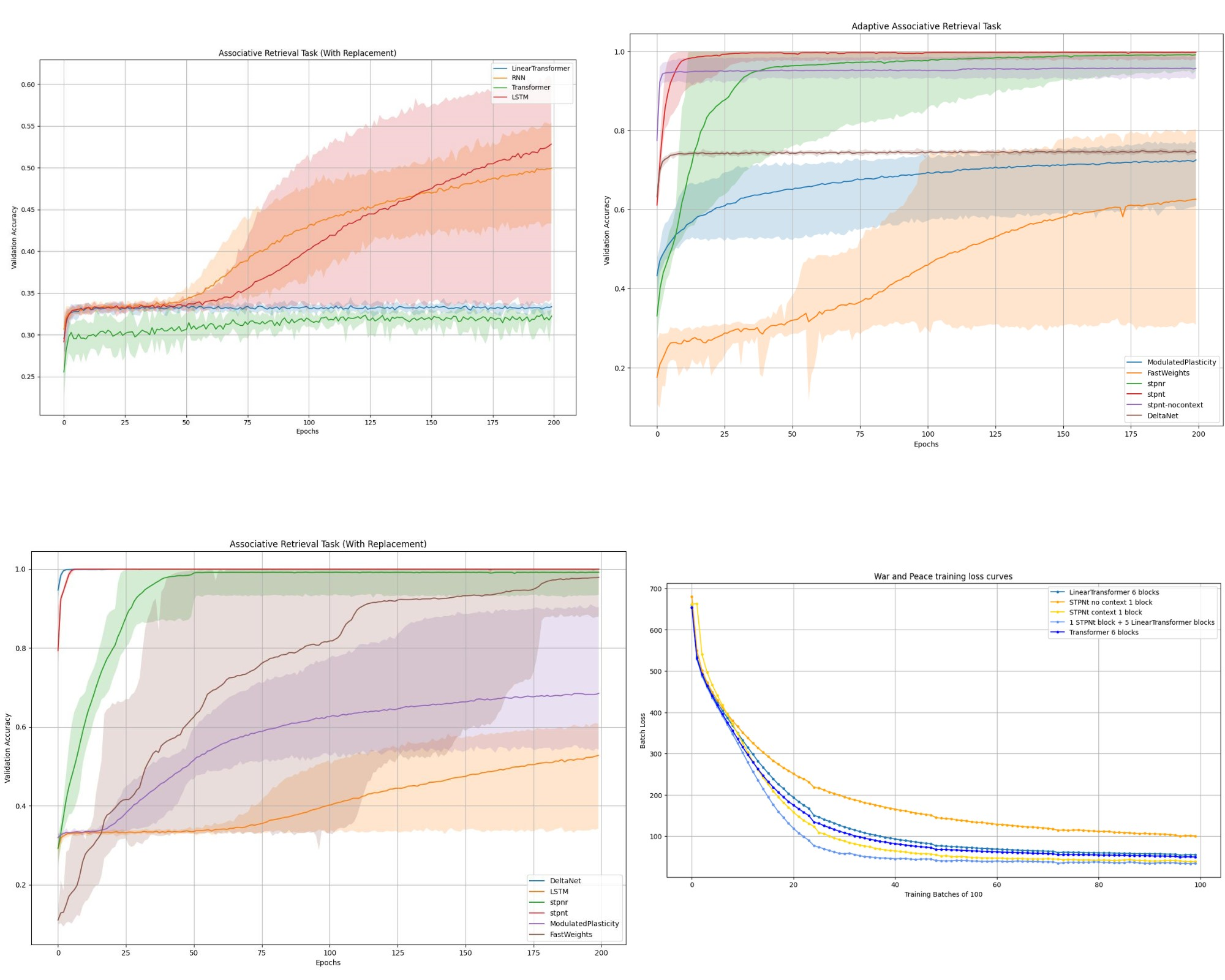
Experimentation was conducted on several toy problems and two datasets: the novel War and Peace, and the language modelling dataset Wikitext-2. In the toy problem, the basic STPNt and STPNt with context were benchmarked against similar models in the literature, as well as the Transformer and Linear Transformer. The results presented in fig. 1 show that the STPNt outperforms the majority of models on both tasks, but performs worse on the toy problem designed to better mimic retrieval in a natural language context. The STPNt with context was introduced here, and showed superior performance to the basic STPNt. This discussion was extended to a language corpus, the War and Peace novel, which recapitulated the importance of context, with the contextual STPNt greatly outperforming the basic model. The experimentation on War and Peace also revealed another insight: stacking STPNt attention blocks caused training instabilities - instead we discovered that the optimal network architecture involved a single STPNt block stacked with Linear Transformer blocks. Finally, experimentation was conducted using the Wikitext-2 dataset, where we also introduced the final model variant: STPNt-LSTM.
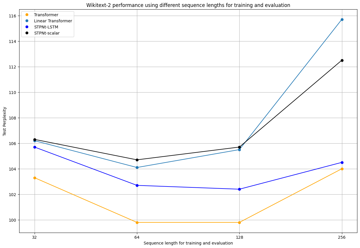
During these experiments, we varied the training and evaluation sequence lengths, and compared the perplexity of the trained models on the test set, shown in figure 3. Surprisingly, the STPNt with context did not provide much benefit over the Linear Transformer, and in fact showed signs of overfitting; lower validation perplexity than the Linear Transformer but higher test perplexity. Nonetheless, the STPNt with context did outperform on sequence lengths beyond 256, and this could be an avenue for further work. The STPNt-LSTM yielded much more positive results: consistently lower training and validation perplexity compared to the Linear Transformer, and demonstrated the ability to utilize longer sequence lengths compared to the Linear Transformer and even the Transformer itself. In fact, the STPNt-LSTM was the only model to achieve a test perplexity improvement from increasing the sequence length from 64 to 128. Knowing that the LSTM cell endows the model with the ability to learn longer sequences, future work could explore the use of an even larger cell state, to see if this could improve things further.
Plastic Parameter Analysis:
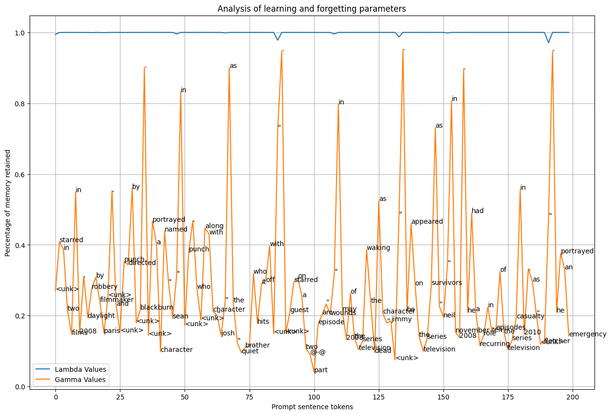
We try to analyse what the STPNt-LSTM is learning by understanding what plastic parameters (lambda, gamma) the model uses when evaluating a a short sequence of text. We include this section to help improve the interpretability of the model,
in the same vein as work done by Kaparthy et al. Using some sample text, we compare the lambda (assigned to modulate the impact of the previous information)
and gamma (modulates the impact of current token) for each token in the sequence.
Through analyzing the results, shown in fig. 4, we see that in fact the lambda parameters are almost unused; for most timesteps, the value of lambda is very close to one, which indicates an incredibly slow decay rate,
which allows for long context. The model does not reset the sequence at any point, but since the sequence is only 128 tokens long, additional analysis needs to be done on longer text, specifically between different topics and articles.
One token that seems to encourage more forgetting of the past are quotation marks, shown by the small dips in the lambda graph. What is more surprising is the model's use of gamma parameters. Here we see that the tokens that the model retains
the most correspond to tokens such as full stops, "in", "as" which are words that appear generally in text, not providing much information about the subsequent tokens. This may be the case due to the small dataset size of Wikitext-2. The model
may not have encountered some words such as names - "Josh" many times, thus not encoding much information in the embeddings of those words, rendering them less useful. However, this is just conjecture, and more work must be done, training on
larger corpuses, such as Wikitext, or the 1 billion words corpus.
We finish our summary by noting several avenues for the continuation of the work in this thesis. Firstly, the models used in the experiments are relatively small compared to those in the literature, and the performance statistics listed
are far from being state-of-the-art, even among non pre-trained models. Thus, one important next step would be to scale up our models, preferably to around 24M trainable parameters which is comparable to the literature, and incorporate
any important regularization techniques. This will be crucial for determining whether our model can truly deliver some benefit. Furthermore, it was discovered upon examining our models parameters during evaluation that the STPNt-LSTM is
learning some counter-intuitive properties of the data, and further work should be done training it on larger language corpuses to explore the consequences of this. Finally, by changing our embedding scheme to a relative one, we could
utilize a "cache" during evaluation time, and this could have interesting effects on the STPNt performance.
The Login App is the first "proper" purely personal project I have taken on. The main objective of this
project was to improve my ability of writing Object-Oriented code. Starting off, I had a basic idea of what I wanted to build -
knowing that along the way I would find more and more features to add and improve on. I chose to use Python, due to it being my
strongest and most used programming language thus far.
I wrote all of the code (which can be found here) using the
AGILE development method - a snippet of my sprint logs is shown below.
The GUI I used for my App was created using a framework built in to the standard library provided
by Python - Tkinter. Using Tkinter sometimes gives the UI a very outdated/clunky look, however, it is easy for new users to pick
up in a short time. The main page, a Tk() object, is the login page (shown below), where existing users can login in. The other pages used by
the app open as Toplevel() objects that "stem" from the login page.
If you are not an existing user, there is an option to register an account with the app. After choosing this option, the user will be asked
to provide several details: a new username, password and email address.
Upon successful registration, an email will be sent to your email address, and a success message will be displayed to the user.
The user can now proceed to log in to the app.
If the username and password both match an account on the system, the app will then prompt the user for a 6 digit code, sent to the
email address they signed up with. (2FA process described in next section)
If the user enters the code correctly, they will reach the landing page of the login app. Here, their username and email address will
displayed. The background is a reference to the TV show Mr. Robot.
This section will talk about the 2 Factor Authentication (2FA) used within the app and the basic security
measures used to make the app more secure, and to protect users. The entire process is very simple, and starts off by concatenating 6 random
integers into a code and sending this to the user's email address, whilst simultaneously prompting the user to enter the aforementioned code.
Then, these can simply be compared - resulting in successful login if they are same, and rejecting sign in if otherwise. In order to add
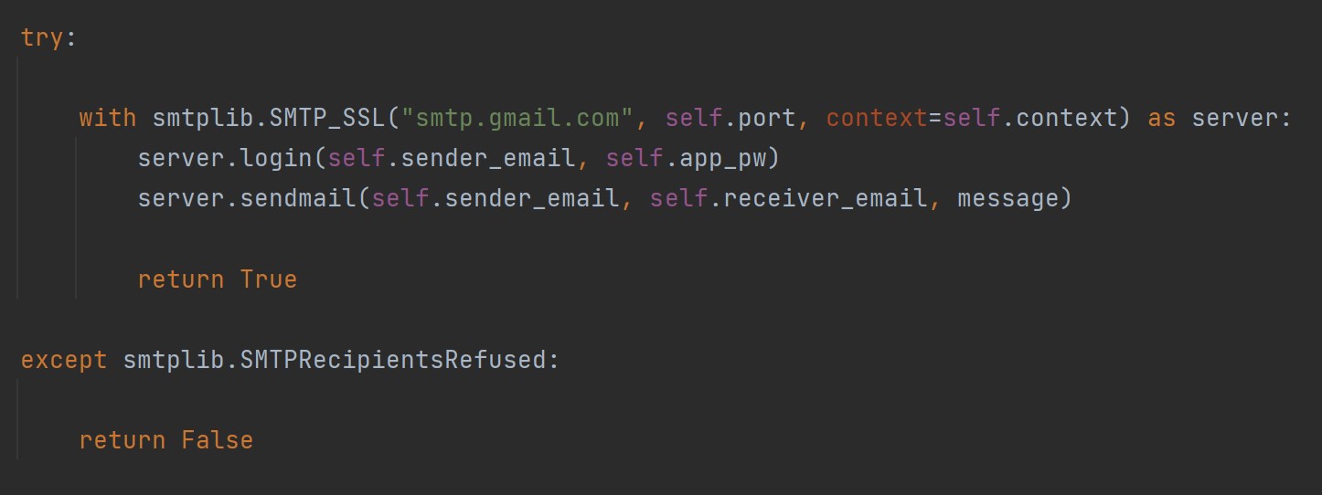
2FA to the app, discovery work was done into sending emails using the built in Python library, smtplib. In particular, I used the class
smtplib.SMTP_SSL(); the code for the mail sending function is shown below.
I will now briefly describe the process carried out by this code.
A link is established to a Simple Mail Transfer Protocol (SMTP) server, here the
specific one used is owned by Google, the address being: "smtp.gmail.com". After using method .login(), and providing correct details to a valid
gmail account, an email can be sent. The email and other details, such as recipient's address is sent over to the host address corresponding to the
SMTP server. The SMTP server will then contact the DNS server in order to find the recipient's IP address.The SMTP server finally sends the information
to email recipient's Mail Transfer Agent (MTA) server. Then, using either POP or IMAP protocols (depending on recipients email client) the email
will arrive at the recipient's inbox. The whole process is done using Secure Sockets Layer (SSL) protocol, which creates an encrypted
connection, making sure that in the unlikely case the email is intercepted midway, hackers cannot access the information within the email.
Aside from 2FA, the app requires users to create a password that adheres to standard requirements:
If the user fails to meet these requirements, the app will reject the password and prompt the user to strengthen the password.
Additionally, passwords that are stored on the database are hashed using SHA-256. This adds extra steps for a hacker that gets access
to the database. If they try to brute force the password, they will need to apply the hash every attempt in order to find the correct
password, which is more time consuming. The algorithm is described in more detail in the next section.
This section will briefly go over the Secure Hashing Algorithm(SHA) - 256, implemented from scratch to be
used to hash passwords in the Login app. Information in this section can be found in its entirety
here, in the pseudocode section.
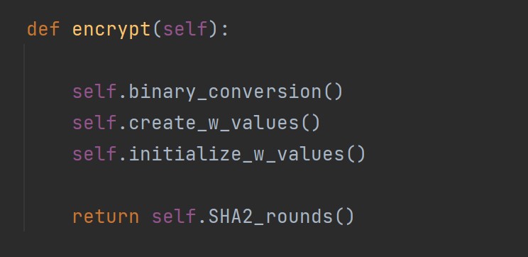
Below, you can see the main method implemented in my class, SHA2, called .encrypt().
Walking through the steps within this method, first there is a method called binary conversion. This simply takes the password string,
and converts each character to binary. Next, the binary string is "padded" with zeros and the message length (also in binary) so that
we end up with a 512-bit binary string.
The next two steps are very related, so they shall be described together. In SHA-256 hashing, there are 64 so called W values, which
are used in "rounds". The first 16 W values, labelled 0 to 15, are created using your initial message, splitting up the 512-bits into
16 x 32-bit chunks. Then, after these have been obtained, the algorithm will proceed to iterate 64 minus 16 times to "generate" the rest
of the W values. This is using the formula below:
Which uses functions for right rotate (switching order of bits) and right shift (removing bits and padding with zeros), as well as existing
W values to find new W values. After this is completed, 64 "rounds" will commence.
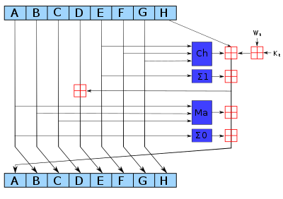
The diagram of a single round is shown below.
A to H at the top represent "working variables". Using a number of different functions: maj, conditional, Sigma, combined with our W values
and K values (created using cube roots of first 64 prime numbers) using modular addition, these working variables are then used to initialize
the working variables of the next round. This is repeated 64 times to retrieve the final set of working variables. Adding these to the initial
working variables and converting to hexadecimal, and finally concatentating, we retrieve the SHA256 hash.
Unittests were written to test the validity of hash function.
SQLite3, built - in to the standard python library was used to connect/create/maintain the database for the Login app. Queries to the database were written in SQL.
This project was completed as part of an assignment for one of my final year modules, "Machine Learning
for Physicists". The final grade achieved for this module was 82%. The objective of this project was to explore methods for classifying
detector images. Traditionally, detector images are pored over by teams of scientists at particle colliders in order to determine what
useful information can be extracted. However, as technology has improved, detectors spit out thousands, if not, millions of images per day.
This is when it becomes unfeasible to check each image individually. So this is where machine learning can come in handy.
My exploration of the different tools available to handle this task were documentated, and presented in the form of a scientific paper. I have
attached the final paper below for you to peruse:
Coming soon