Spectral clustering is a clustering algorithm which is often used in graph theory to separate nodes into distinct groups.
It does this in three main steps. Firstly, we extract an adjacency matrix from the graph. There are different ways of constructing this
matrix, but the underlying ideas remain the same. The adjacency matrix, as the name suggests, describes which nodes are "neighbouring" or
in close proximity to each other. This can be done in a discrete (nearest neighbours) or a more continuous way (using a RBF kernel). Using
this matrix, we can construct a graph Laplacian matrix. The Laplacian matrix of a graph describes many of its important properties, e.g. the sparsest
cut of the graph is approximated by the Fielder vector, which corresponds to the eigenvector related with the second smallest eigenvalue.
Second, we find the spectral decomposition (eigen decomposition) of the Laplacian matrix to retrieve the eigenvalues (spectrum) and corresponding eigenvectors. The eigenvectors are termed spectral
embeddings, which are often used reduced dimension embeddings of the original points. These eigenvectors also have a physical meaning - if we imagine the Laplacian matrix as a
"transformation" of the basis vectors, then the eigenvectors represent certain unit vectors on the space which are not "knocked" off their span. In other words,
eigenvectors are only multiplied by a constant factor when the Laplacian matrix is applied to them. Most choices of adjacency matrix result in symmetric Laplacian
matrices, so the resulting eigenvectors also form a new basis.
Finally, using these spectral embeddings, we can divide up the original points into a specified number of clusters, k. The most common method is to use
the K-means algorithm on the embeddings.
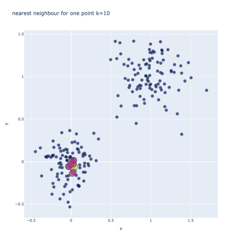
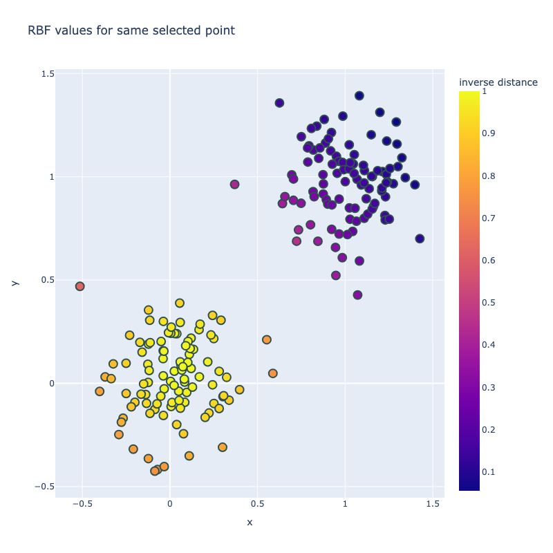
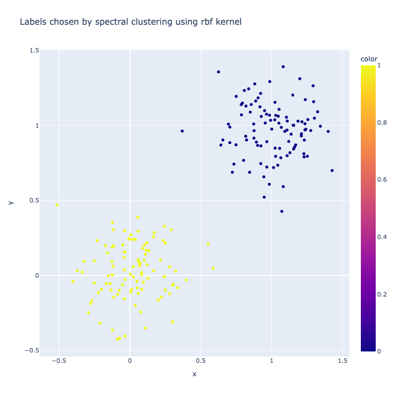
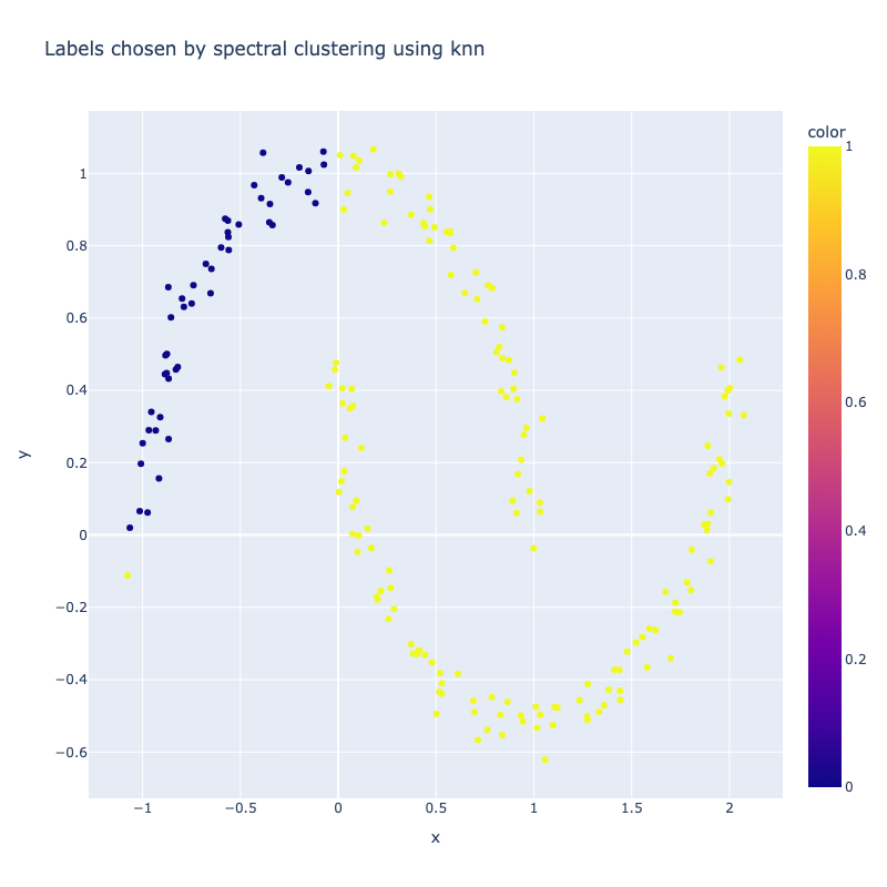
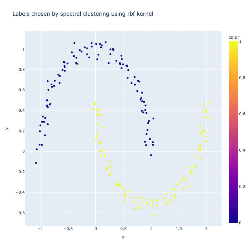
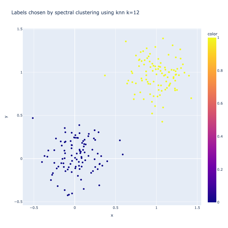
I implemented a spectral clustering algorithm using only numpy and the K-means function from sklearn. I trialled the two adjacency matrix mentioned above, on a simple problem, then a harder one to compare their performance. Both adjacency matrix methods are quite sensitive to hyperparameter values. The tuning process has been abstracted away, using a qualitative trial and error to find a value which classifies the most nodes correctly. Below are the results. It can be seen that the RBF kernel provides an advantage over the nearest neighbours approach, which misclassfies half of one crescent in the harder two moons problem, which is erroneously assigned to the wrong class due to its proximity to the tip of the other crescent. This is unsurprising, as by using nearest neighbours, we are essentially dropping important information about the n - k other nodes.
Coming soon
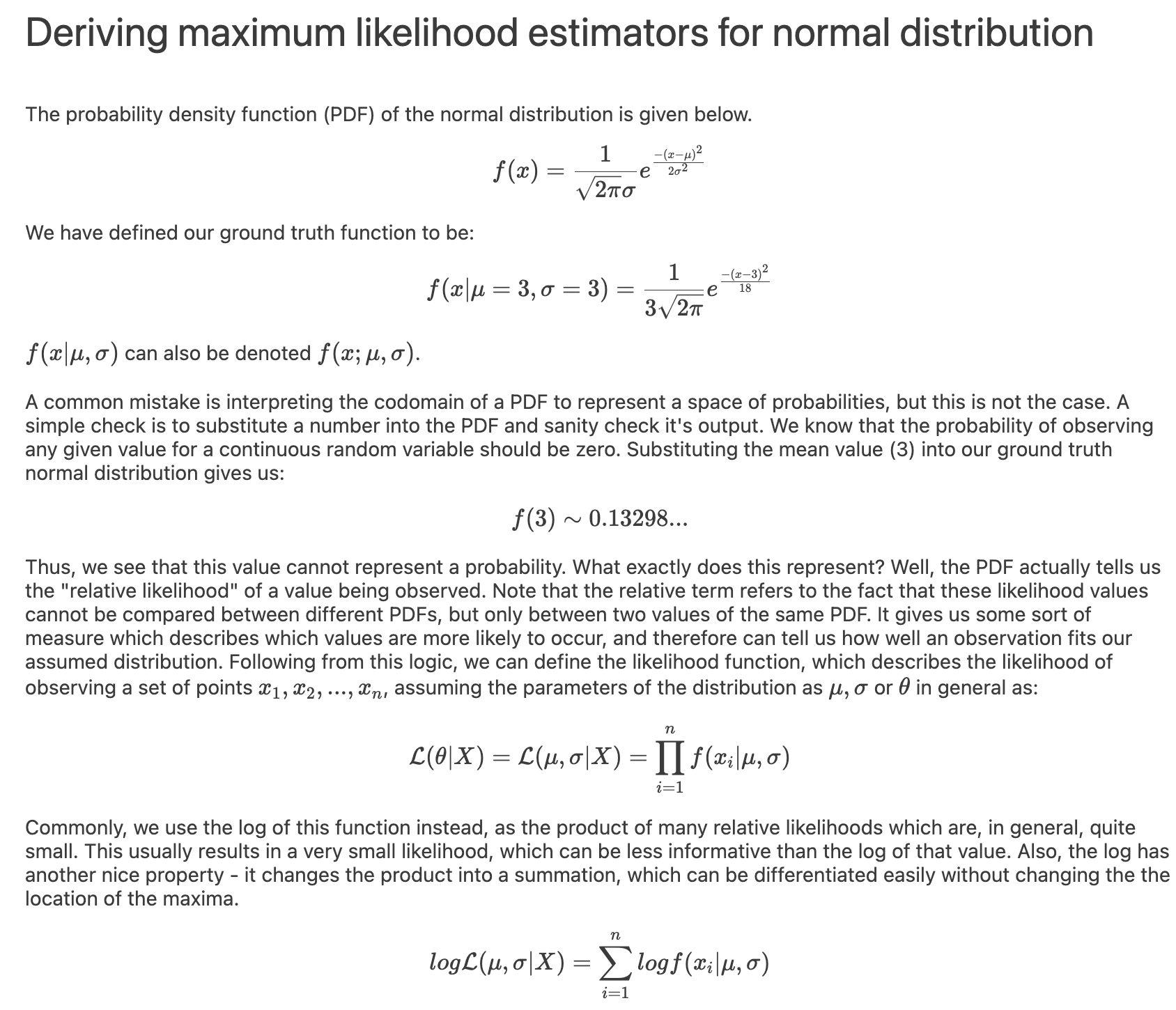
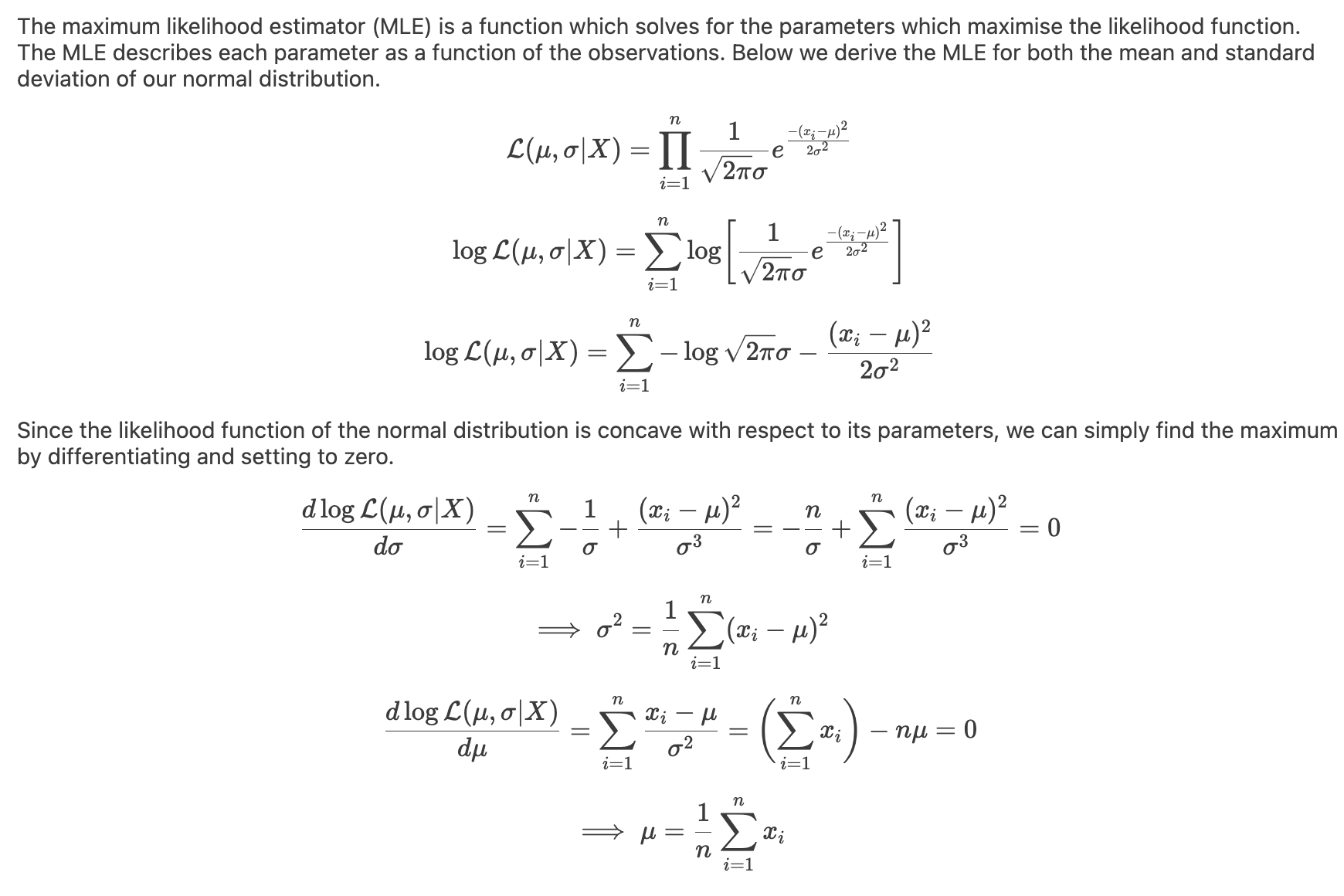
Maximum likelihood estimation (MLE) is a frequentist approach to inferring model parameters from a dataset. Firstly, we assume that data has been drawn from a particular distribution. This
choice of distribution is key as it can bias the results or provide a bad fit. Using the chosen distribution, we then require some observations/data through experimentation or using
historical data. Distributions are often characterized by certain model parameters, such as the standard deviation and mean for the normal distribution. Assuming an arbitrary set of parameters,
we can find an expression for the total likelihood of having observed our dataset. Using this expression, the next step is to find the "most likely" set of
parameters by maximizing the likelihood expression for each of the parameters (differentiating and setting to zero).
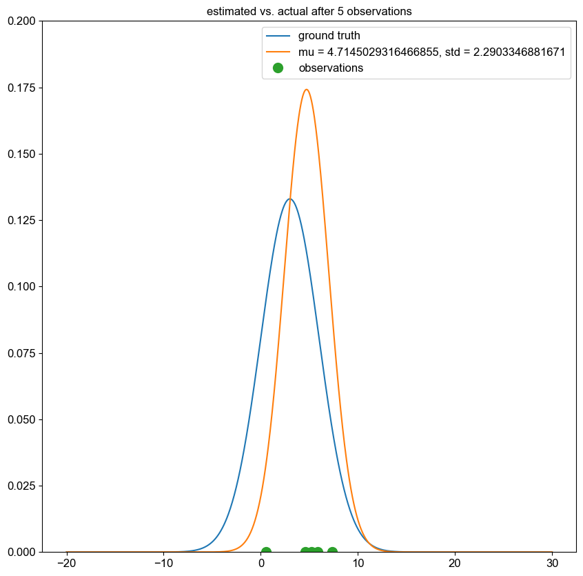
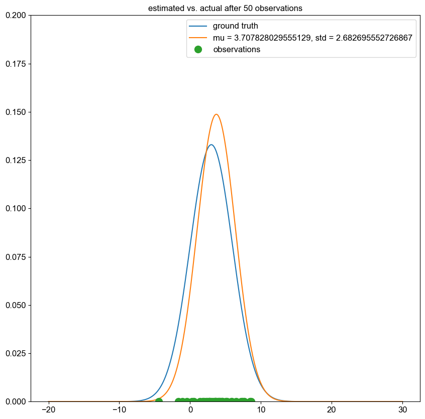
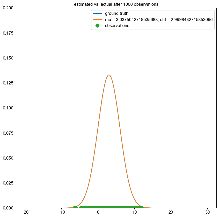
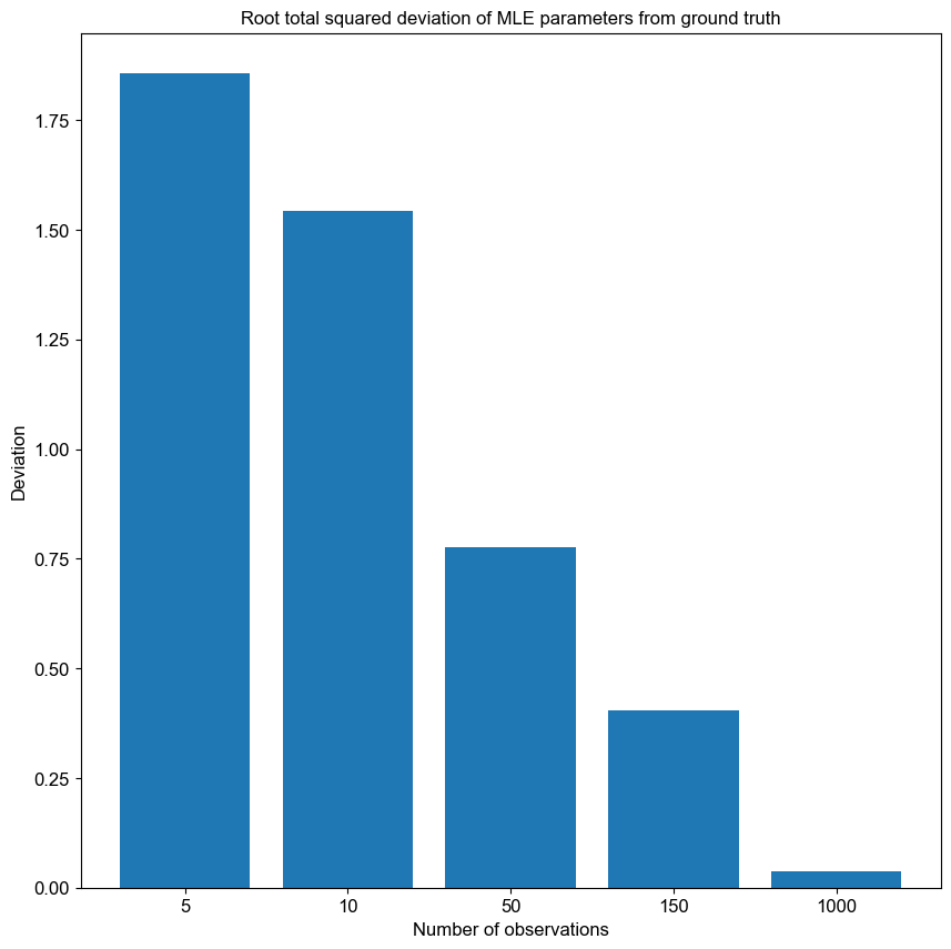
Below are some screenshots from a Jupyter notebook I created, which works through the basic application of maximum likelihood estimation for a univariate normal distribution, where we generate points using
a normal distribution with known parameters and attempt to fit another normal distribution using the outlined MLE methodology.
After progressively more observations, we can see that the estimated parameters from MLE approaches the true underlying distribution.
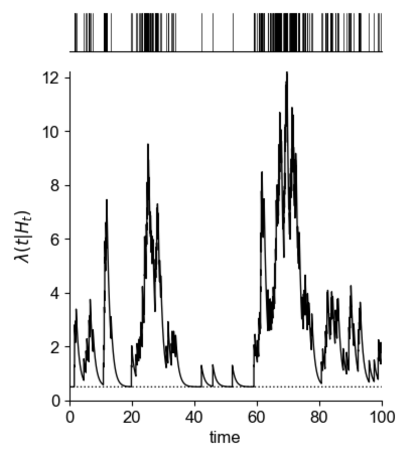
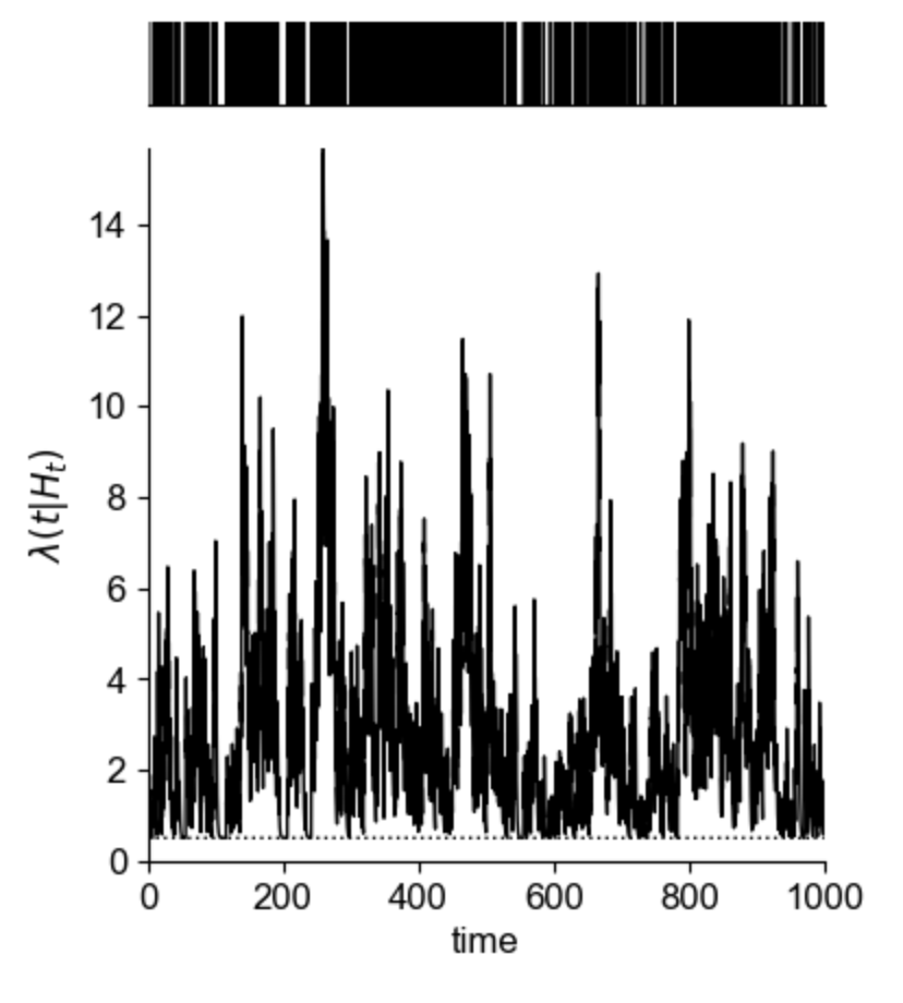
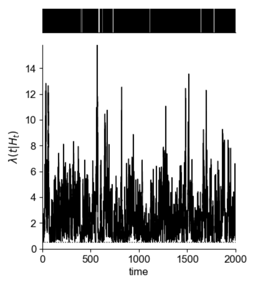
For my research into continuous temporal network analysis, one common model that I have to do parameter fitting for is a Hawkes process, a bursty point process. This
particular model assumes self-exciting events, which means an event instantaneously increases the probability of another event occurring after, decaying over time. For this
model, we follow the same framework as for the normal distribution, with the caveat that we can no longer analytically solve the maximum likelihood estimator due to the
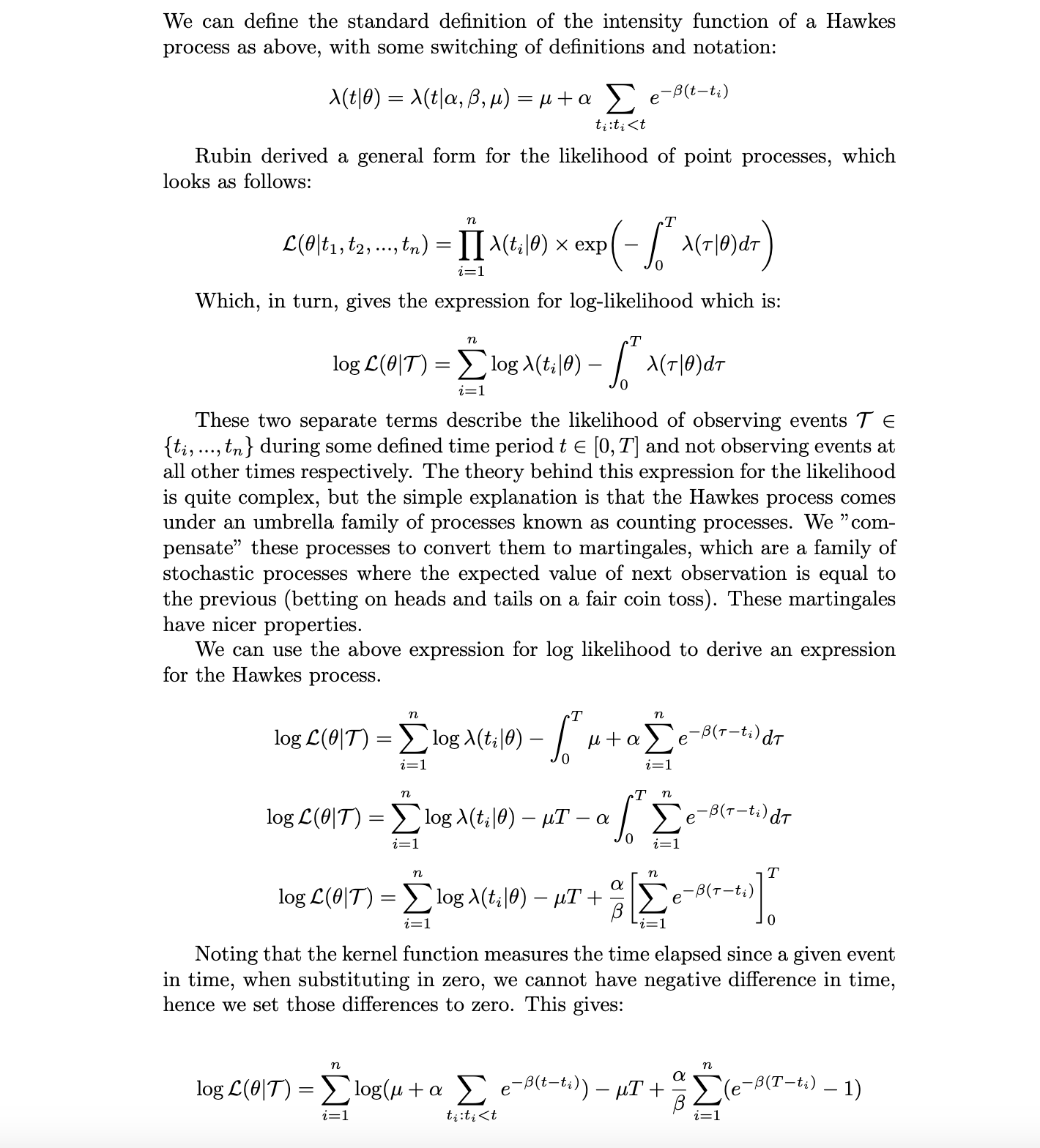
expressions being non-linear. In this case we can employ non-linear optimization methods, such as Newton-Raphson, Powell or LBGS. Again, I provide screenshots of the
derivations.
There are various different methods for non-linear optimization. Some methods will require the further derivations of the gradient with respect to each parameter, and some
even require the hessian matrix for optimization. For simplicity, we use the Nelder-Mead algorithm which only requires the functional value of the log likelihood
at each iteration. We utilise the scipy optimize library to run the optimization and we use the Hawkes library
created by Omita Kahiro to simulate data generated from a hawkes process. Unlike the normal distribution, instead of providing more observations, we instead run the simulation for
longer periods, allowing the model more events to learn the process dynamics from. We use an underlying hawkes process with mu equal to 0.5, alpha equal to 0.8, and beta equal to 1.
These correspond to the baseline rate, jump size and decay strength respectively.
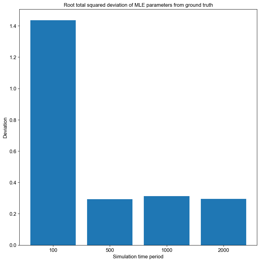
As we can see, the trend in deviation of the parameters is less pronounced here, and it seems somewhere between a simulation of 100 to 500 there was a sharp increase in estimation accuracy, hence the drop in deviations. We also notice that the simulations must be quite high variance, as we see a small increase in deviation from 500 time steps to 1000. This is indeed the case as one event occurring can impact the rest of the simulated time period, leading to drastically different patterns of events for the same hawkes model with same parameters.